When data stays in discontinuous cells, how do you select and copy the data? It will waste a lot of time to select all discontinuous cells with data one by one, especially the data stay in nearly random order. The following tricky way will help you select call cells with data in selections quickly.
Select all cells with data excluding formulas with Go to Special command
If there is not data calculated with formula, the Go to Special command can help you select all cells with data in selections easily.
Step 1: Select the range that you will work with, and then press F5 key to open the Go To dialog box.
Step 2: Click the Special button to get into Go To Special dialog box. Then check the Constants option, see screenshot:
Step 3: Click OK, then you will see all cells with contents excluding the formula cells are selected.
Note: This way is not able to select cells with formulas.
Select all cells with data including formulas with VBA code
If you have cells filled with formulas, you can select all cells with data in selection with the following VBA code. Please do as this:
Step 1: Hold down the Alt + F11 keys in Excel to open the Microsoft Visual Basic for Applications window.
Step 2: Click Insert > Module, and paste the following macro in the Module Window.
VBA code: select all cells with data including formulas
Step 3: Then press F5 key to run this code, and a prompt box will pop out to tell you to select a range that you want to select the data cells.
Step 4: After selecting the range, then click OK, and all the data cells including formulas in the range has been selected.
Select all cells with data including formulas with one click of Kutools for Excel
If you want to select the cells contain data both values and formulas with just fewer steps, here, I can introduce you an easy way, Kutools for Excel, with its Select Unblank Cells feature, you can select the data cells just a few clicks.
After installing Kutools for Excel, please do as follows:( Free Download Kutools for Excel Now )
Step1: Select the range that you want to select only the data cells.
Step2: Click Kutools > Select > Select Nonblank Cells, and then all the cells with data have been selected at once, see screenshot:
If you have piles of data in an Excel worksheet and need to insert cells, rows or columns in the middle of that worksheet then it is possible to add them without starting the worksheet from the beginning all over again. The most abhorrent way to insert cells, rows and columns is to going through all troubles and start over from the beginning again. In this guide, we will how you how to insert cells, rows and columns using the latest and older versions of MS Excel.
When you add a new blank cell in the middle of a worksheet then MS Excel shifts the position of the existing rows and columns accordingly to place the new cell in the spreadsheet. Currently the limit of rows is a little over one million and the limits of columns is a little under seventeen thousands which is more than enough even if you are working in a spreadsheet for business purpose. Here’s how to add a new blank cell in a worksheet.
- Part 1: How to Insert New Cells on A Spreadsheet
- Part 2: How to Insert New Rows on A Spreadsheet
- Part 3: How to Insert New Columns on A Spreadsheet
Part 1: How to Insert New Cells on A Spreadsheet
Step 1. Choose the cell or numbers of cells where you want to add new cells. Meaning if you want to add ten new cells then select ten cells on the worksheet.
Step 2. If you want to terminate any selection then simply click on any cell from the worksheet to cancel the selection.
Step 3. Next, go to the Home tab and click on “Insert” from the Cells category.
Step 4. Now, click on “Insert Cells” to continue.
Step 5. You will have to choose in which direction you want to push the surrounding cells and click on insert.
Alternatively, you can select a cell or a range of cell and then right-click and click on “Insert“. After you finish up the settings, you should be able to see that the new cells are inserted on the exact position that you have selected and the surrounding cells are shifted according to the command you have set.
Part 2: How to Insert New Rows on A Spreadsheet
If you want to insert a new row then first you will have select the row or a cell in a row above where you want to insert the new row. For example, if you want to insert a row above row right then select the eighth row or a cell in the eighth row. After that, follow this instruction to insert a new row.
Step 1. Select the row and right-click on it and click on “Insert“.
Step 2. Alternatively, you can click on Home tab and then click on “Insert” from the Cells group category.
Step 3. Next, click on “Insert Sheet Rows“.
Additional Tip: If you want to insert more than one row then select the multiple rows above where you want to add those new rows and follow the same procedure as mentioned above.
Now, you can adjust the whole worksheet automatically or you can manually choose where to shift the existing rows. You can either adjust them cell reference according to your choice or leave it to the default settings.
NOTE: if you’ve been working with MS Excel every day, you must set a password to protect your excel document. If you forgot MS Excel password, try Office Password Recovery tool to recover your forgotten Excel password.
Part 3: How to Insert New Columns on A Spreadsheet
To insert a new column, simply select the exact right side of the column where you want to insert the new column. For example, if you want to add a new column to the left of fifth column, then select the fifth column and use the following procedure to add a new column.
Step 1. Select the column or a range of column and right click on it followed by clicking on “Insert“.
Step 2. Alternatively, click on Home tab and then choose “Insert” from the Cells group.
Step 3. Click on “Insert Sheet Columns” and adjust the settings of the adjacent columns.
Additional Tip: To insert multiple columns, simply select the numbers of columns or a range of columns that you want to add and follow the same procedure mentioned above.
Please Note: If you want to repeat the same action again and again then simply press CTRL + Y simultaneously to keep adding rows or columns on the worksheet.
Conclusion:
As you see how simple it is to insert new cells, rows and columns in a worksheet. It will be incogitable to create a new worksheet from the beginning just to add few rows or columns instead you should use the mentioned methods to save time and work efficiently. The method is applicable to all new and older versions of Microsoft Excel.
Vicky is a professional Windows technology author with many experience, focusing on computer technology. She’s very much enjoy helping people find solutions to their problems. Her knowledge and passion always drive her to discover everything about technology.
How to unlock your Windows 7 Password without reinstallation
What should I do if I forget my password for iTunes backup,
How to recover lost or forgtten password for Windows 8
What to Do If You Forgot or Lost Windows 10 Login Password
If you need to organize data in a tabular form, there is nothing better than doing that in a spreadsheet. When it comes to spreadsheet programs, Microsoft Excel is the most popular one, however, Google Sheets has also earned a lot of popularity among a number of users in the recent days for the flexibility to work on it from anywhere. But even after organizing everything in a tabular form, you sometimes need to print the same out, which can be done by the conventional method. Depending upon the number of tables, you might need several sheets of paper to print the entire spreadsheet.
However, at times, you might need to print a part of the spreadsheet, and you can do that with both Microsoft Excel and Google Docs by tweaking a small setting at the time of printing the spreadsheet. Apart from printing, the tutorial will also be applicable, if you want to save a certain part of a spreadsheet as a PDF document, using a PDF printer. The ability to print certain parts of a spreadsheet can surely come in handy in a number of real-life situations, both for your official, as well as your personal requirements.
So, without any further delay, let’s get started with, how you can print a certain area of a spreadsheet using Microsoft Excel and Google Docs.
Print selected cells in Microsoft Excel
Step 1: Open the spreadsheet on Microsoft Excel, which you are going to print, and select the cells within the spreadsheet that you want to print.
Step 2: After you have selected the cells that will be printed, click on ‘File’ and then on ‘Print’ . Alternatively, you can use the universal shortcut key, i.e. ‘ Ctrl + P ’ to get the ‘Print’ dialogue.
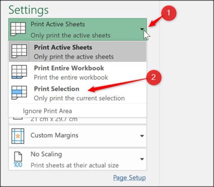
Step 3: In the ‘Print’ dialogue, click on the first drop-down menu under ‘Settings’ , and select ‘ Print Selection ’. By default, the selected option will be ‘ Print Active Sheets ’. After you have made the selection, a preview will be displayed on the right side of the screen. If you are satisfied with the preview, just click on the ‘Print’ button.
You will get only the cells that you have selected, printed on a piece of paper. However, if the selected set of cells is too big for one page, it will require more pages to get the selected set of cells printed.
I have used Microsoft Excel 2019 for this tutorial. However, the process will hardly vary, on the older versions of Microsoft Excel, as well.
Print selected cells in Google Docs
The process is similar if you are using Google Docs, as well.
Step 1: Just select the set of cells that you want to print on the spreadsheet selected by you.
Step 2: Now, click on ‘File’ , and then click on ‘Print’ . Just like the previous case, you can use the ‘ Ctrl + P ’ shortcut key, as well.
Step 3: After the Print dialogue appears, just select ‘Selected cells’ from the drop-down menu under ‘Print’ . The selected range of cells will also be displayed to you. A preview will be displayed to you, just like it was, in the case of Microsoft Excel. After you are satisfied with the preview, click on ‘Next’ .
Finally, you will have to select the printer, and other system-specific settings to print the selected set of cells on a piece of paper.
So, it is really easy to print a selected set of cells both in Microsoft Excel and Google Docs. This will really be useful in your everyday life. Do you have any questions? Feel free to comment on the same below.
There are times when you need to print out data from Excel. But often times you don’t need to print out the entire report which wastes paper, ink, and time.
There will be many times when you need to print out Excel spreadsheets at the office or home office. But oftentimes, you really don’t need to print out the entire report, which wastes paper, ink, and time. Here’s how to print out only the specific areas of the spreadsheet that you need.
Print Select Areas of Excel Spreadsheets
Start by opening the Excel spreadsheet you need, hold down the Ctrl key and highlight the area of the document you want to print out.
After selecting the area you want to print out, go to Page layout > Print Area > Set Print Area.
You won’t really notice anything happen to the document at that point, but next, while still under the Page Layout tab, click Print Titles.
Next, select the Sheet tab in the Page Setup windows that appears. From here, type in the Columns and Rows that you want to repeat (if any), then click on Print Preview. This allows you to include any headers or labels associated with the data.
Now you will get a view of the area you’re printing out. And you can select the printer you want to use and adjust print settings. You can get deep into the printer settings. You can tweak the preview area and manually type in more cells if you want to include them.
If you get too deep into adjusting print areas, they will stay until you clear them out. From the ribbon under Page Layout, click Print Area > Clear Print Area.
This is a great way to save printer ink and paper, as well as time for you and your colleagues. Nothing is worse than someone printing out 500 pages when you need the printer to get one simple page.
Also, remember you don’t need to waste time and ink printing out entire web pages either. If you only want to print out specific info from an article, read our article: How to print only selected text from a webpage.
Sometimes, you may have a large dataset, but you want to print the selected area in Excel on one page. You can do it easily by applying 3 easy methods which we will discuss below. I hope you will soon get rid of issues to print selected area in Excel on one page after reading this tutorial.
Download Practice Book
Download the following Excel file for your practice.
3 Easy Methods to Print Selected Area in Excel on One Page
Here, we have a dataset in an Excel worksheet. Our goal is to print the selected area in this worksheet on one page.
1. Print Selected Area in Excel on One Page Using File Tab
The easiest way to print a selected area on one page is to use the File tab. You just need to follow the steps below.
Steps:
- Select the area that you need to print. Here we have selected B4:F12.
- press CTRL+P.
Or, click the File tab from the top-left corner of the window.
- Click Print.
- Now, click on the first option in Settings.
- Select the Print Selection.
- Lastly, click on the Print button. It will print only the current selection of the page.
Here is the printed page,
2. Print Selected Area in Excel on One Page Using the Page Layout tab
Another easy way to print specific areas in an Excel worksheet is to use the Page Layout tab. Just follow the steps below.
Steps:
- Select the range of cells D5:F12 or the area you want to print out.
- Go to the Page Layout tab > the Print Area drop-down > the Set Print Area option.
- Now, click Print Titles under the Page Layout. A Page Setup window will pop up.
- Go to the Sheet Click on Print Preview. You will see a preview of the specific area that you want to print.
- Now, select the printer you want to use from the Print option of the File
- Click on the Print button.
Note:
The print area that you set will be saved when you save the Excel workbook. If you want to clear the selected area, then click Print Area under Page Layout, Select Clear Print Area.
Similar Readings:
3. Add Cells to an Already Selected Print Area
You can add new cells to your previous selected print area (In this case, we will add all the cells of the column titled “First Name” to our previous method’s print area). For this, you need to follow the steps below.
Steps:
- Select the cells that you need to add to the current print area.
- Go to the Page Layout tab > the Page Setup group > the Print Area drop-down > the Add to Print Area option. Now, after saving the workbook, the print area will be saved.
If you want to view all the print areas, click View> Page Break Preview from the Workbook Views group.
Note:
If the cells that you need to join are not adjacent to the current print area, another print area will be created. Each print area in a worksheet will be printed separately. Only adjacent cells can be adjusted to a current print area and can be printed on one page.
Conclusion
In this tutorial, I have discussed 3 easy methods of how to print selected area in Excel on one page. I hope you found this article helpful. You can visit our website Exceldemy to learn more Excel-related content. Please, drop comments, suggestions, or queries if you have any in the comment section below.
How do I print a specific range in Excel?
Select and highlight the range of cells you want to print. Next, click File > Print or press Ctrl+P to view the print settings. Click the list arrow for the print area settings and then select the “Print Selection” option. The preview will now show only the selected area.
How do you define a range in open office?
Defining your Ranges click on Data → Define range… You will see the range that you have selected highlighted in the background. Give a name to the range designated in the Range field. If the range isn’t what you want, click the icon next to the Range field and select another range.
How do I set print area in open office?
Setting the area to be printed
- Go to the desired sheet.
- Click and drag to select (highlight) the area of the sheet to be printed.
- Select Format – Print Ranges – Add from the main menu.
- Repeat the above steps for each sheet of the file to be printed.
Which option is used to print a particular range of cells from a sheet?
On the worksheet, click and drag to select the cells you want to print. Click File > Print > Print. To print only the selected area, in Print Options, click Current Selection.
How do I print a range of cells?
On the worksheet, select the cells that you want to define as the print area. Tip: To set multiple print areas, hold down the Ctrl key and click the areas you want to print. Each print area prints on its own page. On the Page Layout tab, in the Page Setup group, click Print Area, and then click Set Print Area.
How do you name a range on a calculator?
Choose Insert – Named Range or Expression.
- Define. Opens a dialog where you can specify a name for a selected area or a name for a formula expression.
- Insert. Inserts a defined named cell range at the current cursor’s position.
- Apply. Allows you to automatically name multiple cell ranges.
- Labels.
How do you create a range of cells on a calculator?
Defining Database Ranges
- Select the range of cells that you want to define as a database range.
- Choose Data – Define Range.
- In the Name box, enter a name for the database range.
- Click More.
- Specify the options for the database range.
- Click OK.
How do I print a table in open office?
Go to the desired sheet. Click and drag to select (highlight) the area of the sheet to be printed. In the drop-down menus, go to Format > Print Ranges > Add. Repeat the above steps for each sheet of the file to be printed.
How do I print portraits in open office?
How do I get Sheet1 to print as portrait and Sheet2 to print as…
- Select Format → Styles and Formatting or press F11.
- Click the Page Styles icon (2nd from the left) in the Styles and Formatting window.
- Right-click in the page style list and select New…
Which Format for a cell name is correct?
The first character must be a letter, an underscore, or a backslash. No spaces are allowed in a range name. The range name should not be the same as a cell address. For example, you can’t name a range U2 or UB40, but BLINK182 and ABBA are just fine.
How do I set print area?
Set one or more print areas
- On the worksheet, select the cells that you want to define as the print area. Tip: To set multiple print areas, hold down the Ctrl key and click the areas you want to print.
- On the Page Layout tab, in the Page Setup group, click Print Area, and then click Set Print Area.
How do you set a row as a print title?
Print row or column titles on every page
- Click the sheet.
- On the Page Layout tab, in the Page Setup group, click Page Setup.
- Under Print Titles, click in Rows to repeat at top or Columns to repeat at left and select the column or row that contains the titles you want to repeat.
- Click OK.
- On the File menu, click Print.
Why is rows to repeat at top greyed out?
If the [Print Titles] button is locked (greyed out), it may be because you are currently editing a cell or you have chart selected. If the “Rows to repeat at top” spreadsheet icon is locked, it may be because you have more than one worksheet selected within your workbook.
What is the range in Calc give example?
In a Calc document, a range refers to a contiguous group of cells containing at least one cell. You can associate a meaningful name to a range, which allows you to refer to the range using the meaningful name.
What is cell range in Calc?
A Cell Range Within a Formula A cell range can be used inside a formula, for example to calculate the sum of the values within the selected cells. The notation for the sum of all values in cell range (A1:C6) is =SUM(A1:C6).
What is cell address in open office?
CELL() returns the absolute address of the referenced cell, as text.
With her B.S. in Information Technology, Sandy worked for many years in the IT industry as a Project Manager, Department Manager, and PMO Lead. She learned how technology can enrich both professional and personal lives by using the right tools. And, she has shared those suggestions and how-tos on many websites over time. With thousands of articles under her belt, Sandy strives to help others use technology to their advantage. Read more.
If you frequently print a certain part of your spreadsheet, you can choose a designated print area in Microsoft Excel. This saves you from having to select it every time you want to print. We’ll show you how.
How to Set a Print Area in Excel
You can set one or more print areas in the same Excel sheet. To set a single print area, select the cells. Then, go to the Page Layout tab and click the Print Area drop-down arrow in the ribbon. Choose “Set Print Area.”
To set multiple print areas in your sheet, hold Ctrl as you select each group of cells.
Here, we selected cells A1 through F13, held the Ctrl key, and then selected cells H1 through M13. Next, head to the Page Layout tab and pick “Set Print Area” in the Print Area drop-down box. When it’s time to print, each print area will display on its own page.
After you set a print area in your Excel sheet, it will save automatically when you save your workbook. This allows you to quickly print that same spot without resetting the print area.
How to View a Print Area
Once you set up your print area, you may want to confirm you’ve selected the right cells. Open the View tab and select “Page Break Preview.” You’ll then see each print area you’ve set for that sheet.
When you finish, click “Normal” or “Page Layout” to return to your sheet, depending on which view you were using.
How to Add Cells to a Print Area
You may need to add more cells to your print area after you set it up. You have two options for adjusting the print area, depending on if you want to incorporate adjacent cells or not.
If you simply want to include another set of cells in the print area setup, select the cells. Then, go to the Page Layout tab and select “Add to Print Area” in the Print Area drop-down box.
When you do this, those additional cells are considered their own print area because they are not adjacent to another print area in the sheet. So, that group of cells will print on their own page as you can see below in the Page Break Preview.
Now if you want to increase the size of a current print area to include more cells, be sure to select the cells adjacent to the area. Then, select “Add to Print Area” in the Print Area drop-down box.
Then if you use the Page Break Preview, you can see that the print area has been increased and stays on the same page.
How to View a Print Preview
If you want to see a quick preview of how the page will look when you print it, return to the Page Layout tab. Click the arrow on the bottom right corner of the Page Setup section of the ribbon.
Click “Print Preview.”
You’ll then see exactly what the sheet will look like when you print. Hit the arrow on the top left to return to your sheet.
Note: Alternatively, you can select File > Print or use a keyboard shortcut, Ctrl+F2, to see your print preview.
How to Clear a Print Area
If you make many changes to your sheet, prefer not to print only a specific section, or want to set up a new print area, you can remove an existing one easily.
Select the print area or a cell within it. Back on the Page Layout tab, click “Clear Print Area” in the Print Area drop-down box.
If you have more than one print area set up, simply do this for each one on your sheet.
For additional help printing in Microsoft Excel, learn how to print the gridlines with row and column headers or how to print an Excel sheet that has a background.
November 25, 2019 by Barbara
Welcome, Excellers to another macro blog in my #MacroMonday #Excel 2019 series. Do you ever wish you could just highlight the selected range of cells in your Excel worksheet, then just print them?. With this small Excel VBA macro, you can. No more selecting a print range or going into print options to just the print the selected range. This code does it automatically for you. Sound like it would be useful and save time?. Good, read on and let’s get writing some simple code.
Preparing To Write The Code.
First, you will need to open the Visual Basic Editor. There are two ways to do this. Either by hitting ALT +F11 or selecting the Developer Tab | Code Group | Visual Basic. Both methods have the same result. You then have a choice, you can either create a module to store your code either in your Personal Macro Workbook or in your current workbook. What’s the difference?. If you save you code in your Personal Macro workbook it will be available for use in any of my Excel workbooks. If you store it in the current workbook then use is restricted to that workbook. As you can see this code will be useful to reuse in any workbook. I will create and save this for future use in my Personal Macro Workbook.
Learn More About Your Personal Macro Workbook (PMW)
If you want to read more about your Excel PMW then check out my blog posts below.
Starting The Macro.
We need to start off the macro by inserting a New Module. Do this by selecting the Personal.xlsb workbook, then Insert Module. Type Sub then the name of your macro. In this example, I have called it simply PrintSelection. Notice that Excel will automatically enter the end text End Sub to end the Sub Routine. We simply need to enter the rest of the code between these two lines.
[stextbox Sub printSelection End Sub [/stextbox]
Printing The Selection.
The next line of simple code simply takes the user-selected range and send it directly to the printer. Be sure to specify how many copied and if you want pages collated if you are printing no
[stextbox Selection.PrintOut Copies:=1, Collate:=True [/stextbox]
Ending The Code.
Once the selection has been printed the code ends. We already have the End Sub piece of code which was already inserted automatically when we started the Macro.
[stextbox End Sub[/stextbox]
Using The Print Selection Macro In Excel.
We have the Excel macro written, but if we want to be able able to use it super effectively then we can either
- Assign a shortcut key
- Add the macro to the Quick Access Toolbar
1. Assign A Shortcut Key.
To assign a shortcut key to your macro selecting
Tools | Macro | Macros and selecting the “Options” button at the bottom. An important point to note is that any key combinations you assign to macros will take precedence over any built-in shortcut keys. Shortcut keys are case sensitive and you can use just the Ctrl key or a combination of both the Ctrl key and Shift key if your letter is uppercase.
2. Add The Macro To The Quick Access Toolbar.
Once you have created your Macro, there are just a few short steps to get attached to a button on the Quick Access Toolbar.
- File – Options- Quick Access Toolbar
- In the Choose Commands From – select Macro
- Select the Macro you want to attach to
- Click Add to move the Macro to a list of buttons on the Quick Access Toolbar
- If you want to replace the Icon then click Modify
- Under Symbol, select the one you want
- Under Display Name – change the name if you want to use a more friendly name
href=”
If you want more Excel and VBA tips then sign up to my monthly Newsletter where I share 3 Excel Tips on the first Wednesday of the month and receive my free Ebook, 30 Excel Tips.
If you want to see all of the blog posts in the Macro Mondays Series or the example worksheets you can do so by clicking on the links below.
We have written previously about printing in Excel 2013, such as this article about how to print all of your columns on one page, but there are many other ways that you can customize the way that a spreadsheet prints. For example, you may find that you only need to print a specific set of rows from your spreadsheet and you want to save the ink and paper that would be wasted by needlessly printing the entire thing. Fortunately it is possible to do this by using the Print Area feature option in Excel.
Only Print Certain Rows in Excel 2013
Aside from saving ink and paper, selectively printing certain rows will make it easier for your spreadsheet’s readers to see the important information in your document. So continue below to learn how to set up your spreadsheet.
Step 1: Open the spreadsheet in Excel 2013.
Step 2: Click the Page Layout tab at the top of the window.
Step 3: Click on the top-most row that you want to print, then drag your mouse down until the desired rows are selected.
Step 4: Click the Print Area button in the Page Setup section of the ribbon, then select Set Print Area.
Now when you open the Print menu, the preview will only show the rows that you just selected. To undo this setting so that you can print the entire spreadsheet, click Print Area again, then click Clear Print Area.
If you want to print specific rows that are not next to each other, then you have a couple of options.
Option 1 – Hold down the Ctrl key on your keyboard and click each row individually. Note, however, that this will result in each row being printed on its’ own individual page, which may not be what you are looking for.
Option 2 – Hide all of the rows that are in between the rows that you want to print, then follow steps 1-4 above to set the print area. You can hide a row by right-clicking on the row number, then selecting the Hide option.
Once you have finished printing, you can then select the visible rows that surround the hidden rows, right-click on the selection, and click Unhide.
If you are working on important documents on your computer, or if you have files that you can’t afford to lose, then it’s a good idea to have a backup plan. A simple way to do this is to purchase an external hard drive to store your backup copies. You can even use a program like CrashPlan to automatically back up your files for free.
For additional ways to customize your printed spreadsheet, consider this article about repeating the top row on every printed page in Excel 2013.
Matthew Burleigh has been writing tech tutorials since 2008. His writing has appeared on dozens of different websites and been read over 50 million times.
After receiving his Bachelor’s and Master’s degrees in Computer Science he spent several years working in IT management for small businesses. However, he now works full time writing content online and creating websites.
His main writing topics include iPhones, Microsoft Office, Google Apps, Android, and Photoshop, but he has also written about many other tech topics as well.
If you print a specific selection on a worksheet frequently, you can define a print area that includes just that selection. A print area is one or more ranges of cells that you designate to print when you don’t want to print the entire worksheet. When you print a worksheet after defining a print area, only the print area is printed. You can add cells to expand the print area as needed, and you can clear the print area to print the entire worksheet.
A worksheet can have multiple print areas. Each print area will print as a separate page.
Note: The screen shots in this article were taken in Excel 2013. If you have a different version your view might be slightly different, but unless otherwise noted, the functionality is the same.
What do you want to do?
Set one or more print areas
On the worksheet, select the cells that you want to define as the print area.
Tip: To set multiple print areas, hold down the Ctrl key and click the areas you want to print. Each print area prints on its own page.
On the Page Layout tab, in the Page Setup group, click Print Area, and then click Set Print Area.
Note: The print area that you set is saved when you save the workbook.
To see all the print areas to make sure they’re the ones you want, click View > Page Break Preview in the Workbook Views group. When you save your workbook, the print area is saved too.
Add cells to an existing print area
You can enlarge the print area by adding adjacent cells. If you add cells that aren’t adjacent to the print area, Excel creates a new print area for those cells.
On the worksheet, select the cells that you want to add to the existing print area.
Note: If the cells that you want to add are not adjacent to the existing print area, an additional print area is created. Each print area in a worksheet is printed as a separate page. Only adjacent cells can be added to an existing print area.
On the Page Layout tab, in the Page Setup group, click Print Area, and then click Add to Print Area.
When you save your workbook, the print area is saved as well.
Clear a print area
Note: If your worksheet contains multiple print areas, clearing a print area removes all the print areas on your worksheet.
Click anywhere on the worksheet for which you want to clear the print area.
On the Page Layout tab, in the Page Setup group, click Clear Print Area.
Need more help?
You can always ask an expert in the Excel Tech Community or get support in the Answers community.
You can quickly locate and select specific cells or ranges by entering their names or cell references in the Name box, which is located to the left of the formula bar:
You can also select named or unnamed cells or ranges by using the Go To ( F5 or Ctrl+G) command.
Important: To select named cells and ranges, you need to define them first. See Define and use names in formulas for more information.
To select a named cell or range, click the arrow next to the Name box to display the list of named cells or ranges, and then click the name that you want.
To select two or more named cell references or ranges, click the arrow next to the Name box, and then click the name of the first cell reference or range that you want to select. Then, hold down CTRL while you click the names of other cells or ranges in the Name box.
To select an unnamed cell reference or range, type the cell reference of the cell or range of cells that you want to select, and then press ENTER. For example, type B3 to select that cell, or type B1:B3 to select a range of cells.
Note: You can’t delete or change names that have been defined for cells or ranges in the Name box. You can only delete or change names in the Name Manager ( Formulas tab, Defined Names group). For more information, see Define and use names in formulas.
Press F5 or CTRL+G to launch the Go To dialog.
In the Go to list, click the name of the cell or range that you want to select, or type the cell reference in the Reference box, then press OK.
For example, in the Reference box, type B3 to select that cell, or type B1:B3 to select a range of cells. You can select multiple cells or ranges by entering them in the Reference box separated by commas. If you’re referring to a spilled range created by a dynamic array formula, then you can add the spilled range operator. For example, if you have an array in cells A1:A4, you can select it by entering A1# in the Reference box, then press OK.
Tip: To quickly find and select all cells that contain specific types of data (such as formulas) or only cells that meet specific criteria (such as visible cells only or the last cell on the worksheet that contains data or formatting), click Special in the Go To popup window, and then click the option that you want.
Go to Formulas > Defined Names > Name Manager.
Select the name you want to edit or delete.
Choose Edit or Delete.
Hold down the Ctrl key, and left-click each cell or range you want to include. If you over select, you can click on the unintended cell to de-select it.
When you select data for Bing Maps, make sure it is location data – city names, country names, etc. Otherwise, Bing has nothing to map.
To select the cells, you can type a reference in the Select Data dialog box, or click the collapse arrow in the dialog box and select the cells by clicking them. See the preceding sections for more options for selecting the cells you want.
When you select data for Euro Conversion, make sure it is currency data.
To select the cells, you can type a reference in the Source Data box, or click the collapse arrow beside the box and then select the cells by clicking them. See the preceding sections for more options for selecting the cells you want.
You can select adjacent cells in Excel for the web by clicking a cell and dragging to extend the range. However, you can’t select specific cells or a range if they’re not next to each other. If you have the Excel desktop application, you can open your workbook in Excel and select non-adjacent cells by clicking them while holding down the Ctrl key. For more information, see Select specific cells or ranges in Excel.
Need more help?
You can always ask an expert in the Excel Tech Community or get support in the Answers community.
At times you may want to print a specific area of a spreadsheet that highlights the salient features you want, rather than bringing an entire worksheet to a meeting. If you want to print a specific part on a worksheet that has the data you want, you can set a print area that includes that specific selection. However, it can be a challenging task if you want to print the same selection on every page of the workbook. In this tutorial you’ll learn:
- What a print area is
- How to set a print area in an Excel worksheet
- How to modify a print area
- How to set a print area on multiple Excel worksheets
Learning how to set a print area on multiple Excel worksheets will not only save you time but will also allow you to print only the information you want.
What a Print Area Is
In Excel a print area allows you to select specific cells on a worksheet which can then be printed off separately from the rest of the page. It simply refers to a range of cells you designate to print when you don’t want to print off an entire workbook.
When you hit Ctrl + P on a worksheet that has a defined print area, only the print area will be printed. You can set multiple print areas in a single worksheet. In this case each print area will print as a separate page.
How to Define a Print Area
Setting a print area is simple and straightforward. Just open an Excel worksheet and highlight the cells you want to print. Click the “Print Area” option on the Page Layout tab, and in the “Page Setup” section select “Set Print Area.”
Keep in mind that the print area will be saved once you save the workbook. Now every time you want to print that worksheet, it will only print the data defined in the print area. To clear the print area, go to the “Page Layout tab -> print area -> clear print area.”
How to Modify Cells in an Existing Print Area
You can modify a print area by adding adjacent cells. Note that the option to add cells will only be visible if you have an existing print area. To add cells to an existing printing area:
1. Select cells that you want to add.
2. Navigate to the Page Layout tab, and on the Page Setup group click Print Area, then select Add to Print Area.
Note: only adjacent cells can be added to an existing print area. If the cells you want to add are not adjacent to the print area, the system will create an additional print area.
How to Create a Print Area on Multiple Sheets
If you use Excel regularly, you have probably created multiple individual sheets in a single Excel workbook. Often you’ll find that some of your workbooks have sheets that are identical in every way save for input data.
For example, a monthly sales report is likely to have around thirty sheets identical in every way except for the figures. Since all the cells are in the same range and alignment, it’s possible to define a print area that will apply to all the other sheets. Let’s look at how to do it.
1. Open your workbook and select the first sheet.
2. Highlight or select the range of cells you want to print.
3. While holding down the Ctrl key, click on each of the other individual sheets you want to print.
4. Click Ctrl + P and then select “Print Selection” in the Print settings. The system is set to print the active sheets by default which means it will print the entire worksheet. Changing that to “Print Selection” ensures you print only the cells that you have highlighted.
5. Click “Preview” to make sure you got it right. Since each print area will print as a separate page, check the number of pages in the preview to ensure all sheets have been captured.
6. Click Okay to print.
Wrapping Up
Defining a print area is a great way to print only the content you want for your presentation. If you want more customization over your printing options, you can try third-party applications such as Kutools for Excel. However, some of the third-party apps are not free and may require a monthly subscription.
Want to become a spreadsheets pro? Check out our article on the 9 add-ons for Excel to make spreadsheets easier.
Our latest tutorials delivered straight to your inbox
MS-Excel is part of the MS-office suite from Microsoft Corporation. It is one of the most popular spreadsheet software in the world. MS Excel worksheet is a huge area full of rows and columns. At times people wish to print only a particular area in a worksheet.
Because a worksheet is massive –the software makers have built-in a logic that it should print only the area that contains data. Print area is by default set to cover all the cells that have some data. If data there is a lot of data Excel will cover it all in print. If you give print command –it will print all the cells. At times you may not need printout of all this.
MS-Excel provides you with the option of selecting a specific area for printing. This saves you from printing unnecessary pages. To set the print are, do as follows:
- Select the area that you wish to print
- Go to Page Layout tab
- Click on Print Are button
- Select “Set Print Area”
The selected area will be marked with distinctive border. You can select and add more print areas –and all the selected areas will be printed in one command. But these areas may not necessarily be on one page.
Following the steps given in the previous section –you will also get option to clear and already set print area. All the print areas will be cleared if you select this option. Also, MS-Excel will automatically calculate and set new print areas as per your printer settings.
We hope that this small tutorial was useful for you. Please feel free to ask should you have any questions related with this topic. We will try our best to assist you. Thank you for using TechWelkin!
By its form, a spreadsheet enables you to spread out and add data to any cell.
However, if you don’t manage your print setup, this can create print jobs with page breaks where you don’t want them and reams of blank pages as Excel works its way down to the random character you entered by accident in cell Z2647.
The Print Area feature in Excel is a powerful tool that makes it easier to print just the data you need by allowing you to select part of a spreadsheet to print.
Check out the products mentioned in this article:
Microsoft Office (From $139.99 at Best Buy)
MacBook Pro (From $1,299.99 at Best Buy)
Lenovo IdeaPad 130 (From $299.99 at Best Buy)
How to set print area in Excel
For the sake of this example, we use a small set of data about employees of a fictitious company. The dataset includes position, division, city, and date of hire. You could sort and print the data multiple ways. You might want a list with just the employees hired before or after a certain date, everyone in a certain position, or employees of a certain division.
We sorted employees by city and selected just those located in Atlanta to print. Here’s how to do that using the Print Area button.
1. Click on “Page Layout” in the top menu to open its menu ribbon.
2. Highlight the cells you want to print by clicking on the first cell and holding down shift on your Mac or PC keyboard while clicking the other cells.
3. Click on the “Print Area” button in the top menu. Choose “Set Print Area.” Hit “Enter” or “Return” on your keyboard to set the print area.
How to check the print area in Excel
1. When you click “File” in the top menu bar and the “Print,” you’ll see a preview of what Excel will print. This will help you determine if you set the right print area correctly.
2. You can also check your print area in the “Page Setup” window in the top menu.
3. Click on the “Page Setup” button. A window will pop up with several ways you can modify your page setup.
4. Click on “Sheet” on the right.
5. The first field under the Sheet tab is “Print Area.” This field displays your print area, starting with the top box on the left and ending with the bottom box on the right.
6. You will also see a moving dotted line around the area you selected to print.
7. If you want to change your print area, click the icon on the right of the “Print Area” field and then highlight the cells you want to print. Now you can print that specific by clicking the File tab and selecting the “Print” option from the drop-down menu.
Pro tip: when you finish printing, click the “Print Area” button again and choose “Clear Print Area.” Otherwise, your spreadsheet tab will retain the print area you selected and the next time you go to print data you’ll get only that limited data, unless you set a new print area.
Hello,
I am trying to set up a few macros that will select a set of cells, select the print option, select print only selection and then press print. I am getting this 1004 error when I try to enact the macro. Here is the debug:
The debugger highlights the second line of code.
Any help is greatly appreciated!
Re: Macro to print selected range of cells
Welcome to Ozgrid. We’re glad to have you on board, however, please note the following regarding thread titles:
Thread titles are used in searching the forum, therefore, it is vital they be written to accurately describe your [COLOR=”blue”]thread content or overall objective[/COLOR] using ONLY search friendly key words. That is, your title used as search terms would return relevant results.
- The title must not use non-essential words such as:”Help needed”, “Formula problem”, “Please help”, “urgent”, “Code issue”, “Need Advice”, etc. Such words dilute the title/search results.
- The title should not contain VBA code or formula syntax or use abbreviations, jargon, delimiters (e.g. slashes, commas, colons, etc)
- The title should not contain reference to VBA error messages as these are too generic to define the specific problem
- The title should not assume or anticipate a solution as in referencing Excel functions or VBA methods – the actual solution is often quite different
- The title should not contain special characters such as
! @ # $ % ^ & * ( ) or math operators – these are not search friendly
Your title of “[COLOR=”red”]Runtime Error 1004 Application or Object defined error[/COLOR]” does not describe your thread or objective and is not helpful to those searching the forum for a solution to a similar need.
[COLOR=”darkred”]Please note the change to your title, which is based on the objective stated in your thread.[/COLOR]
If the new title still does not accurately describe your thread you may make further edits as needed per the above guidelines.
———————————————————-
Also,
All VBA code posted in the forum must be wrapped in code tags, which you omitted, including single-line code snippets.
I’ve added the tags for you this time only. Be sure to use them in future posts.
[COLOR=”navy”]How to use code tags[/COLOR]
Print in VBA is very similar to the print in excel, when we have important data in excel or spreadsheets then the only way to have them safe is to save them to pdf or print them, for print we need to set up the print command in VBA first before using it, what this command does if prints or writes the data into another file.
Table of contents
- What is Print in VBA Excel?
- Syntax of VBA PrintOut in VBA Excel
- Examples of Print in VBA Excel
- Parameters of Printout Method in VBA Excel
- How to use the Parameters of Print Out Method in Excel VBA?
- Recommended Articles
What is Print in VBA Excel?
After all the hard work we have done to present the report to the manager, we usually send emails. But in some cases in the meeting, your manager needs a hard copy of your reports. In those scenarios, you need to print the report you have in the spreadsheet. One of the reasons your manager needs a print out of the report could be a very large report to read on the computer. In a worksheet, you must have already familiar with printing the reports. In this article, we will show you how to print using VBA coding. Follow this article for the next 15 minutes to learn how to print reports in VBA.
Syntax of VBA PrintOut in VBA Excel
Before we see the syntax, let me clarify this first. What do we print? We print ranges, charts, worksheets, workbooks. So PrintOut () method is available with all these objectives.
[From]: From which page of the printing has to start. If we don’t supply any value, it will treat as from the first page.
[To]: What should be the last page to print? If ignored, it will print till the last page.
[Copies]: How many copies you need to print.
[Preview]: Would you like to see the print preview before proceed to print. If yes, TRUE is the argument, if not FALSE, is the argument.
You are free to use this image on your website, templates etc, Please provide us with an attribution link How to Provide Attribution? Article Link to be Hyperlinked
For eg:
Source: VBA Print (wallstreetmojo.com)
Examples of Print in VBA Excel
Below are the examples of Print in VBA Excel.
For illustration purposes, I have created dummy data, as shown in the below picture.
Now we need to print the report from A1 to D14. This is my range. Enter the range in the VBA code to access the PrintOut method.
Code:
Now access the PrintOut method.
Code:
I am not touching any of the parameters. This is enough to print the selected range. If I run this code, it will print the range from A1 to D14 cell.
Parameters of Printout Method in VBA Excel
Now I have copied and pasted the same data to use other parameters of the PrintOut method in VBA Excel.
When we want to print the entire sheet, we can refer to the entire sheet as Active Sheet. This will cover the entire sheet in it.
Code to Print the Entire Worksheet.
Code:
Code to Refer the Sheet Name.
Code:
Code to Print all the Worksheets in the Workbook.
Code:
Code to Print the Entire Workbook Data.
Code:
Code to Print Only the Selected Area.
Code:
How to use the Parameters of Print Out Method in Excel VBA?
Now we will see how to use the parameters of the print out method. As I told, I had expanded the data to use other properties.
For sure, this is not going to print in a single sheet. Select the range as A1 to S29.
Code:
Now select the print out method.
Code:
The first & second parameters are From & To, what is the starting & ending pages position. By default, it will print all the pages, so I don’t touch this part. Now I want to see the print preview, so I will choose Preview as TRUE.
Code:
Now I will run this code. We will see the print preview.
This is coming in 2 pages.
So first, I want to set up the page to come in a single sheet. Use the below code to set up the page to come in one sheet.
Code:
Like this, we can use VBA print out a method to print the things we wanted to print and play around with them.
Recommended Articles
This has been a Guide to VBA Print Statement. Here we discuss how to use Excel VBA Code for printout along with examples and step by step explanations. You can learn more about Excel VBA from the following articles